TYMPANOMETRY / IMPEDANSOMETRY

Standard clinical tympanometry is usually performed with a low frequency stimulus at 226 Hz (or 220 Hz). At low frequencies, the normal middle ear system is stiffness-controlled and susceptance (stiffness element) contributes more to overall admittance than conductance (frictional element). Other typical probe tone frequencies include 678 Hz (or 630, 660 Hz), 800 Hz, and 1000 Hz. Typically static air pressure is varied from +300 daPa to -300 daPa. The direction of pressure change (i.e. from positive to negative pressure or vice versa) may influence static admittance (Wilson et al., 1984). At higher frequency probe tones (e.g. 678 Hz) notched tympanograms are more frequent with
increasing pressure change (Wilson et al., 1984). Also, the rate of pressure change can have an effect on tympanograms. Single-peaked tympanograms typically increase in amplitude with increasing rates of pressure change, but also the incidence of multiple-peaked tympanograms increases (Creten and van Camp, 1974). Moreover, the incidence of notches increases with successive runs of tympanometry measurements maybe due to the viscoelasticity of the tympanic membrane.

The result of the admittance measurement is a graph called a tympanogram which plots middle ear admittance as a function of static air pressure in the outer ear canal (see Figure 68). Different middle ear pathologies exhibit different tympanogram shapes. The following rough description refers to low frequency (226 Hz) tympanograms. In case of normal middle ear function the tympanogram shape corresponds to a Gaussian bell curve with its maximum being around zero static pressure (black solid line), i.e. maximum energy is transferred into the middle ear at atmospheric pressure without any static pressure offset. If there is a Eustachian tube dysfunction the peak of the Gaussian bell curve is shifted in the direction of negative pressure values (red dashed line). This is due to the fact that the tympanic membrane moves best in its normal position, i.e. when the static pressure in the ear canal
and the static pressure in the tympanic cavity are the same. If the static pressure in the tympanic cavity is negative then the static pressure in the outer ear canal has to be negative with the same value. As a result, the peak of the Gaussian bell curve is present exactly at the static pressure which is obtained in the tympanic cavity. In case of middle ear effusion, middle ear mass is increased. In this case middle ear movement is considerably reduced resulting in a lower compliance (light blue dotted line), which is nearly independent of static pressure. Also, in case of otosclerosis middle ear movement is reduced. As a consequence, the peak of the Gaussian bell curve is small, however located within the zero static pressure range (gray solid curve). An activated stapedius muscle yields
reduced compliance as well.

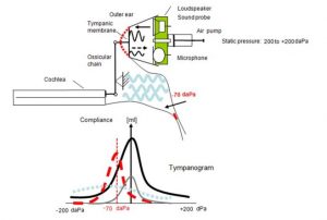
Figure 1: Schematic overview of tympanometry (top) with tympanogram examples (bottom: black solid line: normal; gray solid line: otosclerosis; red dashed line: Eustachian tube dysfunction; light blue dotted line: effusion).

Typical parameters from a tympanogram are the tympanometric shape, ear canal volume, static admittance, tympanometric peak pressure, and tympanometric width. Jerger and Northern (1980) introduced three types of tympanogram shapes, which refer to low frequency (226 Hz) tympanograms. Type A represents a normal tympanogram with a pronounced peak around 0 daPa, Type B shows a flat tympanogram without pronounced peak, and Type C refers to tympanograms with the peak shifted to negative static pressure. For low probe tone frequencies commonly a single-peaked tympanogram occurs. However, in neonates and for higher probe tone frequencies tympanograms often exhibit multiple peaks and notches (dependent on which immittance component is measured).
Ear canal volume is typically estimated as the admittance at the negative or positive maximum pressure (e.g. at +200 daPa). For low frequency probe tones only a small error occurs due to a phase difference between the admittance vector of middle ear and ear canal. At higher frequencies, this error becomes more prominent. For a 226 Hz probe tone, the ear canal volume is commonly given in ml (which is similar to mmho at this frequency and at specific environmental conditions). For higher frequency probe tones, the ear canal volume is given in mmho. The tympanogram can be normalized by subtracting the ear canal volume from the curve yielding the compensated static acoustic admittance Ytm, which is an estimate of the acoustic admittance at the lateral surface of the tympanic
membrane. It is typically higher when maximum negative (rather than maximum positive) pressure is used to estimate ear canal admittance (Margolis and Smith, 1977). The tympanometric peak pressure is the pressure at which the maximum admittance occurs. The tympanometric width is the pressure difference at one half of the compensated static acoustic admittance. It quantifies the relative sharpness of the peak.

PRACTICAL USE
Select Tymp from the module selection screen. The Tymp module can be found in the Immittance section. Select the preset that you would like to perform. If necessary, change the parameters (e.g. minimum/maximum pressure, speed of pressure change, probe tone frequency, auto start, auto stop, reflex options) and the preset name as required.

The tympanometry test can optionally be performed with consecutive automated acoustic reflex testing. If you wish to perform an acoustic reflex test immediately after tympanometry select reflex options in the tympanometry settings accordingly.
Make sure that a valid transducer (tympanometry ear probe EP-TY) is connected to the device and check that the air tube connector is tightly screwed on the pressure outlet socket of the device (see Figure 2). You may use a clip to fix the ear probe cable to the subject’s clothes. Select an ear tip with appropriate size matching the probe tip size and the subject’s ear canal size. Make sure that the ear probe is inserted without any leakage between ear probe and ear canal. Foam tips are usually not suitable for performing tympanometry because they are not airtight

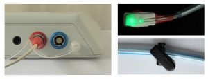
Figure 2: Tympanometry setup (left: attaching the tympanometry ear probe EP-TY to a Sentiero Desktop device; top right: EP-TY status light, bottom right: fixation clip)

After selecting the test ear, the measurement is ready to be started. The ear probe status light indicates the current measurement condition:
– Steady light: Ready for testing – please place the ear probe in the ear
– Slowly blinking (heartbeat): Measurement in progress
– Fast blinking: Leakage, unable to generate the required pressure in the ear canal
The device continuously monitors the probe fit, i.e. the acoustical volume seen at the ear probe (see Figure 3).

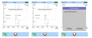
Figure 3: Monitoring of probe fit for tympanometry (left: invalid probe fit when starting the test; middle: valid probe fit when starting the test; right: invalid probe fit during test)

The tympanometry measurement starts automatically (if configured) once the ear probe is appropriately positioned in the ear canal and the acoustical volume has stabilized. The ear probe status light indicator will change from steady to heartbeat mode while the admittance curve is recorded. In case of leakage during the test, a message box appears asking the user to commence or cancel the test. The ear probe status light will change to fast blinking, and instructions will appear on the device display. The device will periodically retry to continue the measurement automatically. During the tympanometry measurement the following information is provided on the screen (see
Figure 4):

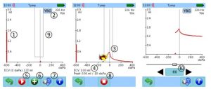
Figure 4: Tympanometry measurement (left: before measurement; middle: during measurement with cartoon mode enabled; right: manual measurement)

Before a test is started manually (if auto start option is disabled), the estimated ear canal volume (ECV) is continuously displayed as bar on the left side of the tympanogram graph ①. The numeric ECV value ④ is additionally shown below the tympanogram graph. For class 1 tympanometers, the tympanogram view mode (admittance Y, conductance G, and susceptance B) can be switched by pressing the YBG button ②. As soon as the tympanometry measurement starts (either automatically if the auto start option is enabled or after pressing the play button ⑤), the admittance as a function of the applied static pressure offset range is plotted as tympanogram ③. If the cartoon mode is enabled, a plane moves along the tympanogram trace. The cartoon mode is especially meant for
focusing a child’s interest and hence improving noise conditions during a test. If a peak is detected, the peak amplitude and static pressure offset is displayed below the ECV estimate ④. A gray box in the middle of the tympanogram graph represents the normal area ⑨. If the tympanogram peak is located within this area, the tympanogram can be expected to be normal. An ongoing measurement can be stopped by pressing the stop button ⑧.

After the test is finished, the tympanometry result is shown (see Figure 5).

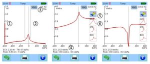
Figure 5: Tympanometry result (left: Admittance with subtracted ear canal volume; middle, right: admittance and conductance for 1000 Hz probe tone)

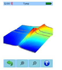
Figure 6: Tympanometry 3D result view

The tympanogram is shown as red (right ear) or blue trace (left ear). The resolution of the ml/mmho axis can be adjusted by swiping a finger up or down the screen. A vertical bar at the left side of the tympanogram graph represents the ear canal volume (ECV) ①. The numeric value of the ECV is shown below the tympanogram graph together with the tympanometric width (TW, for 226 Hz probe tones only), and the peak amplitude and static pressure offset ④. The normative area is shown as gray box ②. For class 1 tympanometers, admittance, susceptance and conductance graphs can be toggled via the YBG button ③. For 226 Hz probe tones, the tympanogram can be shown normalized by subtracting the estimated ear canal volume from the trace yielding the compensated static
acoustic admittance Ytm (= admittance of the tympanic membrane alone). The probe tone frequency and view mode are indicated in the upper right corner. For multi-frequency measurements you can chose to plot the tympanogram for each probe tone frequency by pressing the respective small admittance graph ⑥. When pressing the 3D tympanogram graph ⑤ (not available in firmware 2.2), a 3D plot calculated from the traces at the four probe tone frequencies is shown (see Figure 6). You can rotate the 3D plot by sliding a finger horizontally or vertically over the screen. By pressing the magnifying glass buttons you can zoom in or out of the graph.